Data Cleaning in Python

After data extraction/collection, the data needs to be cleaned before analysis. Data cleaning is an important task in data science since the collected data can have many problems including incorrect data format, missing data, incorrect input values, and so forth. This task covers more than half of the overall task in Data Science. Today, we will look at some of the important concepts in the data cleaning process.

Simple Data Cleaning

Some essential functions used in data cleaning includes:

#(if the DataFrame is named as df)
df.isnull()

This returns a Boolean table indicating True when the value is null and False otherwise

df.notnull()

This does the reverse of isnull() i.e. return True when the value is not null and False when null

df.dropna()

This drops the rows when any of its value is null. We can drop columns too by assigning the parameter axis = 1. By default, the function drops the rows(or columns) when any single value is null, we can also set the function to drop the row(or column) if all of its value is null by assigning the parameter how='all'.

df.fillna(0)

This fills all the null values in the DataFrame with the value of 0. Any other value can be set apart from 0.

Another important aspect is renaming the columns in the DataFrame. At times, the column name is too complex and renaming it can simplify our task. This can be achieved with the rename method of the dataframe.

df.rename(columns = {'old_name': 'new_name'}
         index = {'old_name': 'new_name'})

The rename method can take two arguments, columns (to rename the column) and index (to rename the row). Each of these takes on a dictionary stating the old name to be renamed and the new name. We’ll see its use in later examples.

Further grouping and data transformation needs to be done to make our data cleaner for analysis. We will look at these concepts with an example dataset.

We will look at the World Happiness Report as an example in all the task that follows. The World Happiness report data can be available here.

import pandas as pd
import numpy as np

happiness_2015 = pd.read_csv('2015.csv')
happiness_2015.head()

A preview of the report looks like

The columns of the dataset include:

Country – name of the country

Region – the region where the country is located

Happiness rank – the rank of the country in terms of happiness score

Happiness score – the overall happiness score of the country

Standard Error – the standard of the happiness score

Economy, Family, Health, Freedom, Trust, Generosity – the contribution of each of the factor in the overall happiness score for the country

Dystopia Residual- Represents the extent to which the factors above over or under explain the happiness score.

Let’s first rename few of the columns, Economy (GDP per Capita), Health (Life Expectancy) and Trust (Government Corruption)

happiness_2015.rename(columns = {'Economy (GDP per Capita)':             
                                  'Economy',
                                'Health (Life Expectancy)':                                                                 
                                  'Health',
                                'Trust (Government 
                                   Corruption)': 'Trust'})

Data Aggregation

Aggregation is applying a statistical operation to groups of data. It reduces dimensionality so that the DataFrame returned will contain just one value for each group. The aggregation process consists of three sets:

1. Split the dataframe into groups

2. Apply a function to each group

3. Combine the results into one data structure

The groupby operation optimizes the split-apply-combine process. We can break it down into two steps:

1. Create a GroupBy object

2. Call an aggregation function

Let us now apply the groupby to the data above. When we look at the data, we see that we can group the countries based on the region column. Lets see what happens

grouped = happiness_2015.groupby('Region')
print(grouped)

This returns us with the output

This shows that the data has been grouped and return a grouped object. To view the number of elements of each group, we can use the size() method of the groupby object.

print(grouped.size())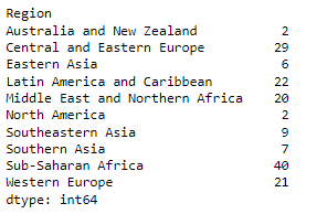

This returns us a series with the number of data (rows) in each group (i.e. region in the data above).

The power of groupby is seen when we want to apply a statistical function (or any other groupby methods) over the grouped data.

Various aggregating fuctions are available which includes: mean(), sum(), size(), count(), min(), max(), etc.

print(grouped.mean())

This gives us a DataFrame object with the mean values of all numeric columns.

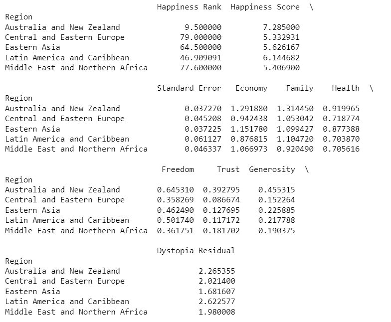
We can also view only a single column or a list of columns by passing the column name to the groupby object.

#selecting single column
print(grouped['Happiness Score'].mean())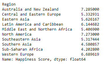

#displaying values for group of columns
print(grouped[['Happiness Score', 'Family', 'Freedom']].mean())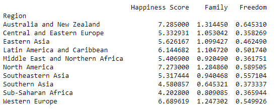

Notice how the index has been set to the column by which the table has been grouped. This can be reset with the reset_index method.

print(grouped[['Happiness Score', 'Family', 'Freedom']].mean().reset_index())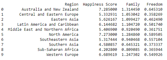

The groupby object also has a agg() method which allows user to pass multiple aggregating function in a single go. However, it should be noted that the function should be passed as a parameter without parenthesis in the agg method.

print(grouped['Happiness Score'].agg([np.min, np.max, np.mean]))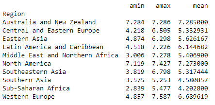

We can also pass a group of columns to apply the aggregate function like in the previous example.

The grouping of data is useful while finding errors in the dataset and some unexpected or unreasonable data that appears in the dataset.

Transforming Data

Many a times there arise situations while cleaning data that we have to apply certain cleaning process (functions) to every row of the data. We can do this by looping through each data and apply the function to each row. Pandas offer a better way to achieve this task through the functions map() and apply(). Both these functions apply the specified function element wise in the series.

For the Happiness report from above example, if we look at the data, there are columns which represents the factors of impact on the overall happiness score. We can convert these rows into category which represents ‘High’ and ‘Low’ impact. For this, we first define a custom function which separated the high and low impact value.

def impact(element):
    if element > 1:
       return 'High'
    else:
       return 'Low'

We then apply this impact function over each row of a column (Series) with the Series.map() and Series.apply() function.

happiness_2015['Family _map'] = happiness_2015['Family'].map(impact)

happiness_2015['Family _apply'] = happiness_2015['Family'].apply(impact)

Upon inspection, we see that both the map() and the apply() function yields the same result. These function takes an element of a row, applies the specified function, returns the result and then moves to another row. Notice how the function has been called without the parenthesis in both map() and apply(). Also note that both of these functions are methods of a series and multiple columns will not work on multiple columns.

Pandas offer applymap() method for the purpose. With the applymap(), we can apply a function over multiple columns at a single go.

factors = ['Economy', 'Family', 'Health', 'Freedom', 'Trust', 'Generosity']
happiness_rank = happiness_2015[factors].applymap(impact)

print(happiness_rank.head())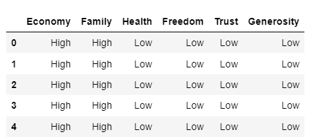

One thing to note is the difference between the apply() and the map() function. Altough, both performs the same task, there is one significant difference between the two. The apply function can take on an argument to be applied. To see this, let’s first create a function which takes two parameters.

def impact_new(element, x):
    if element > x:
        return ‘High’
    else:
        return ‘Low’

When we apply the above function with the map(), we get an error while apply() can successfully implement it.

happiness_new = happiness_2015['Family'].map(impact_new, x=0.8)

happiness_new = happiness_2015['Family'].apply(impact_new, x=0.8)
happiness_new.head()

The blog has been written as a part of the Data Insight program.

Some of the content has been referred from the DataQuest platform.

Examples of the entire blog can be found in my GitHub repo.