Time Series Analysis of NAICS (North American Industries Classification System)
- Kala Maya Sanyasi
- Jan 20, 2022
- 5 min read
Time series analysis is a statistical technique which deals with time-series data. In time series data the data is in a series of particular time period or interval.
The files from the data set are all flat files that is Excel (.xlsx), and CSV (.csv) files, so we will merge and append data from several files.
For the datasets we have 15 RTRA (Real-Time Remote Access) CSV files, which has employment data by industry, 2-digit NAICS, 3-digit NAICS, and 4-digit NAICS.
First we import the necessary libraries to carry out the data analysis.
import pandas as pd
import numpy as np
import glob
import matplotlib.pyplot as plt
import matplotlib.patches as patches
Then import all the 15 csv files.
file_path = r'G:\DataScience\Data Insight\NAICS\csv_files'
all_csv_files = glob.glob(file_path + '/*.csv')

csv_list = []

for csv_file in all_csv_files:
    combined_dataframe = pd.read_csv(csv_file, index_col = None, header = 0)
    csv_list.append(combined_dataframe)

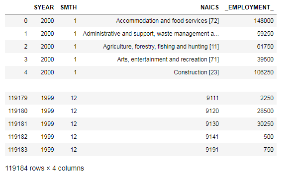
data = pd.concat(csv_list, axis = 0, ignore_index = True)
data
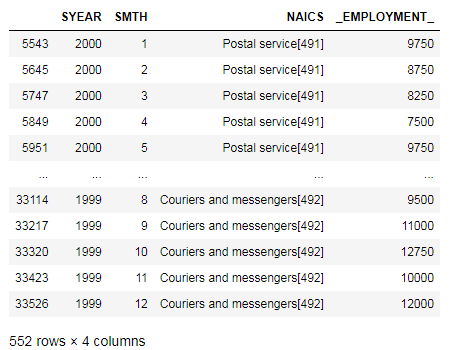
From the data we will couriers and messengers from postal services which contains 492 and save as Couriers_and_messengers.
Couriers_and_messengers = data.loc[data['NAICS'].str.contains('492', na = False)]Do the same for postal service that contains 491
Postal_service = data.loc[data['NAICS'].str.contains('491', na = False)]Now we will concat Postal service couriers and messengers.
Postal_service_couriers_and_messengers = pd.concat([Postal_service, Couriers_and_messengers])

Postal_service_couriers_and_messengers
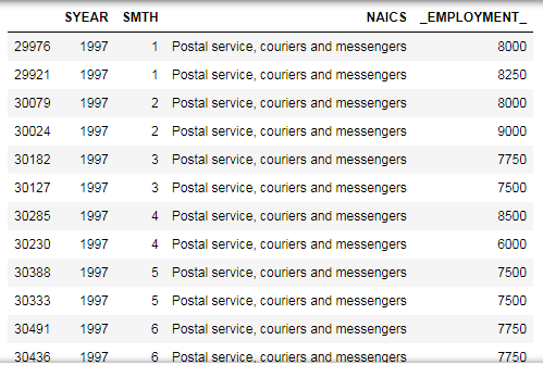
After changing all column names to Postal service, couriers and messengers, the dataframe is sorted by the SYEAR and SMTH columns. Then, the Employment column is segregated to add up consecutives even rows to get the sum of empoyments from both [491] and [492]. After that, the dataframe is merged back and the columns names are changed to reflect our Data Output Template.
Postal_service_couriers_and_messengers = Postal_service_couriers_and_messengers.replace(
    'Postal service[491]', 'Postal service, couriers and messengers')

Postal_service_couriers_and_messengers = Postal_service_couriers_and_messengers.replace(
    'Couriers and messengers[492]', 'Postal service, couriers and messengers')
df1 = Postal_service_couriers_and_messengers.sort_values(['SYEAR', 'SMTH'])
df1.head(50)From df1 we will drop 'SYEAR', 'SMTH', 'NAICS' and save as df.
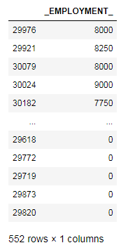
df = df1.drop(['SYEAR', 'SMTH', 'NAICS'], axis = 1)
df
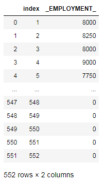
Now we add index
df.index = np.arange(1,len(df)+1)
df = df.reset_index()
df
We filter odd and even.
df = df.set_index('index')
df_odd = df.loc[df.index.values % 2 == 1]
df_even = df.loc[df.index.values % 2 == 0]
df_even = df_even.set_index(df_even.index.values - 1)
new = df_odd.add(df_even, fill_value = 0)
new = new.reset_index().reset_index()
df2 = df1[np.arange(len(df)) % 2 == 0]
df2 = df2.reset_index().reset_index()We merge df2 and drop the columns level_0, index_x, _EMPLOYMENT__x, index_y from Postal_service_couriers_and_messengers.
df3 = pd.merge(df2, new, how = 'inner', on = 'level_0')
df3 = df3.drop(['level_0', 'index_x', '_EMPLOYMENT__x', 'index_y'], axis = 1)
df3.columns = ['SYEAR', 'SMTH', 'LMO_Detailed_Industry', 'Employment']
Postal_service_couriers_and_messengers   = df3

Postal_service_couriers_and_messengers = Postal_service_couriers_and_messengers[
    (Postal_service_couriers_and_messengers.SYEAR != 2019)]
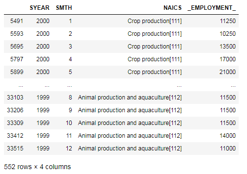
Getting Farms from Crop production[111] & Animal production and aquaculture[112]
Crop_Production = data.loc[data['NAICS'].str.contains('111', na = False)]
Animal_production_and_aquaculture = data.loc[data['NAICS'].str.contains('112', na = False)]
Farms = pd.concat([Crop_Production, Animal_production_and_aquaculture])
After changing all column names to Farms, the dataframe was sorted by the SYEAR and SMTH columns. Then, the Employment column was segregated to add up consecutives even rows to get the sum of empoyments from both [111] and [112]. After that, the dataframe was merged back and the columns names were changed to reflect Data Output Template.
Farms = Farms.replace('Crop production[111]', 'Farms')
Farms = Farms.replace('Animal production and aquaculture[112]', 'Farms')
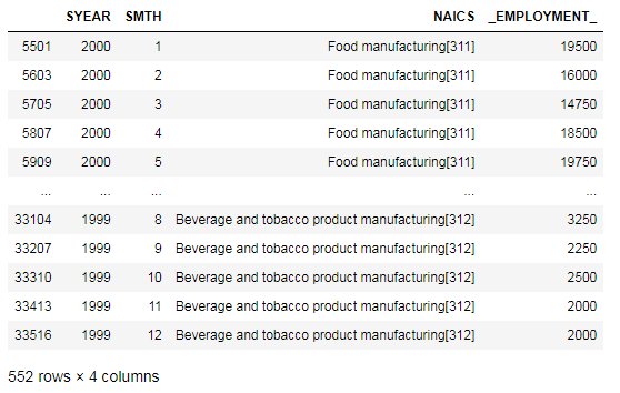
Getting Food, beverage and tobacco manufacturing from Food manufacturing[311] & Beverage and tobacco product manufacturing[312]
Food_manufacturing = data.loc[data['NAICS'].str.contains('311', na = False)]
Beverage_and_tobacco_product_manufacturing = data.loc[data['NAICS'].str.contains('312', na = False)]
Food_beverage_and_tobacco_manufacturing = pd.concat([Food_manufacturing, Beverage_and_tobacco_product_manufacturing])
Food_beverage_and_tobacco_manufacturing
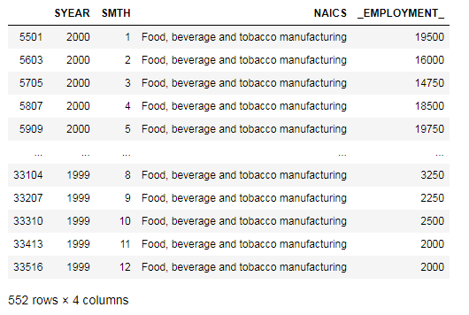
After changing all column names to Food, beverage and tobacco manufacturing, the dataframe was sorted by the SYEAR and SMTH columns. Then, the Employment column was segregated to add up consecutives even rows to get the sum of empoyments from both [311] and [312].
Food_beverage_and_tobacco_manufacturing = Food_beverage_and_tobacco_manufacturing.replace(
    'Food manufacturing[311]', 'Food, beverage and tobacco manufacturing')
Food_beverage_and_tobacco_manufacturing = Food_beverage_and_tobacco_manufacturing.replace(
    'Beverage and tobacco product manufacturing[312]', 'Food, beverage and tobacco manufacturing')
Food_beverage_and_tobacco_manufacturing
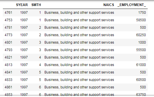
The whole process was repeated to obatin the Business, building and other support services. After changing all column names to Business, building and other support services, the dataframe was sorted by the SYEAR and SMTH columns. Then, the Employment column was segregated to add up consecutives even rows to get the sum of empoyments from both [55] and [56].
MCE = data[data['NAICS'] == 'Management of companies and enterprises [55]']
MCE.SYEAR.value_counts().sort_values()
AWR = data[data['NAICS'] == 'Administrative and support, waste management and remediation services [56]']
AWR_reduced = AWR[(data['SYEAR'] != 2016) & (data['SYEAR'] != 2017) & (data['SYEAR'] != 2018) & (data['SYEAR'] != 2019)]
AWR_removed_data = AWR[(data['SYEAR'] == 2016) | (data['SYEAR'] == 2017) | (data['SYEAR'] == 2018) | (data['SYEAR'] == 2019)]

Business_building_and_other_support_services = pd.concat([MCE, AWR_reduced])
Business_building_and_other_support_services = Business_building_and_other_support_services.replace(
    'Management of companies and enterprises [55]', 'Business, building and other support services')

Business_building_and_other_support_services = Business_building_and_other_support_services.replace(
    'Administrative and support, waste management and remediation services [56]', 'Business, building and other support services')

df1 = Business_building_and_other_support_services.sort_values(['SYEAR', 'SMTH'])
Adding removed data and renaming the coulmns
Business_building_and_other_support_services = pd.concat([Business_building_and_other_support_services, AWR_removed_data])
Business_building_and_other_support_services.columns = ['SYEAR', 'SMTH', 'LMO_Detailed_Industry', 'Employment']

Business_building_and_other_support_services
Data Visualisation
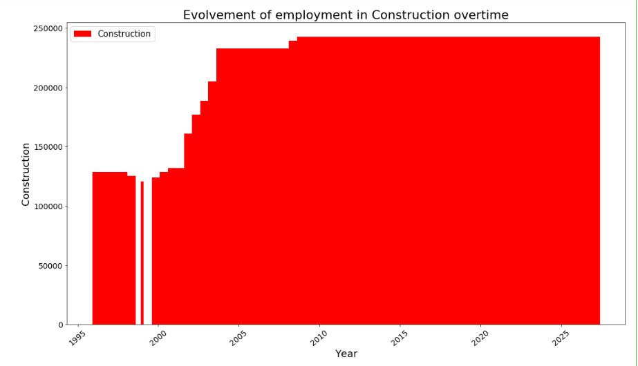
1. How employment in Construction evolved overtime?
plt.figure(figsize=(18,10))
plt.bar(Construction['SYEAR'], Construction['Employment'], color = 'r')

plt.xlabel('Year', fontsize=18)
plt.xticks(rotation=40, fontsize = 14)
plt.ylabel('Construction', fontsize=18)
plt.yticks(fontsize = 14)
plt.title('Evolvement of employment in Construction overtime', fontsize=22)
red = patches.Patch(color='red', label='Construction')
plt.legend(handles=[red], prop = {'size':15})
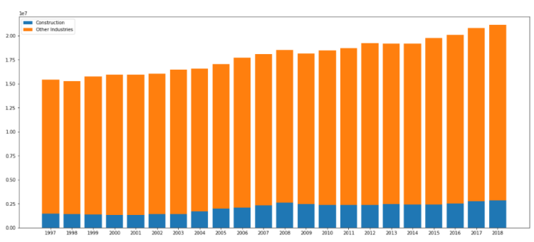
2. How employment in Construction evolved over time, compared to the total employment across all industries?
data_output.loc[data_output['LMO_Detailed_Industry'] == 'Construction [23]'].groupby('SYEAR').sum()['Employment']
data_output.loc[data_output['LMO_Detailed_Industry'] != 'Construction [23]'].groupby('SYEAR').sum()['Employment']
plt.figure(figsize=(14,10))
x_industries = ['1997', '1998', '1999', '2000', '2001', '2002', '2003', '2004', '2005', '2006', '2007', '2008', '2009',
'2010', '2011', '2012', '2013', '2014', '2015', '2016', '2017', '2018']
x_indexes = np.arange(len(x_industries))
width = 0.20
y_construction = [1489750, 1424750, 1363500, 1345750, 1347250, 1401500, 1412000, 1705000, 1989000, 2097000, 2301000, 2616750,
2444750, 2380750, 2365750, 2383250, 2453000, 2406500, 2417750, 2536000, 2743250, 2860750]
plt.bar(x_indexes, y_construction, width = width, label = 'Construction')
y_other = [20344750, 20454250, 20863000, 22305750, 22218750, 22602000, 22585750, 22602000, 23088750, 23592500, 24161500,
24339750, 23966000, 24443500, 24485750, 24895000, 24865750, 25087750, 25415500, 26156250, 27012500, 27220250]
plt.bar(x_indexes - width, y_other, width = width ,label = 'All other companies')
plt.legend()
plt.xlabel('Years of Construction evolvement', fontsize=18)
plt.xticks(ticks = x_indexes, labels = x_industries, fontsize = 12, rotation = 60)
plt.ylabel('Evolvement of Construction employment over time', fontsize=18)
plt.yticks(fontsize = 14)
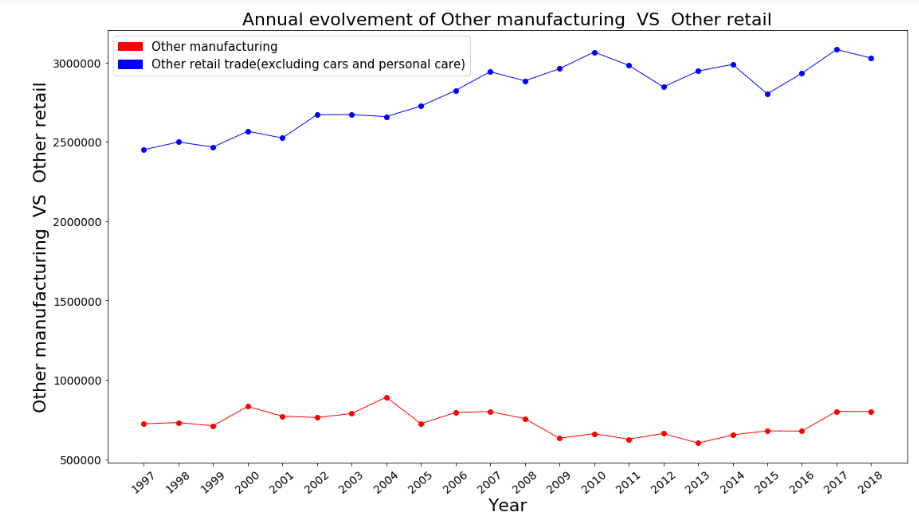
plt.title('Evolvement of Construction compared to All other industries', fontsize=22)3. How employment in Other manufacturing evolved over time, compared to the employment across Other retail trade in terms of month and years?
manufacturing_series = data_output_mixed.loc[data_output_mixed['LMO_Detailed_Industry'] == 'Other manufacturing'].groupby('SYEAR').sum()['Employment'].to_frame()
retail_series = data_output_mixed.loc[data_output_mixed['LMO_Detailed_Industry'] == 'Other retail trade(excluding cars and personal care)'].groupby('SYEAR').sum()['Employment'].to_frame()
years = pd.Series(x_industries).to_frame()
plt.figure(figsize=(18,10))
plt.plot(years[0], manufacturing_series['Employment'], color = 'r',marker='o', linewidth=1)
plt.plot(years[0], retail_series['Employment'], color = 'b',marker='o', linewidth=1)
plt.xlabel('Year', fontsize=22)
plt.xticks(rotation=40, fontsize = 14)
plt.ylabel('Other manufacturing VS Other retail', fontsize=22)
plt.yticks(fontsize = 14)
plt.title('Annual evolvement of Other manufacturing VS Other retail', fontsize=22)
red = patches.Patch(color='red', label='Other manufacturing')
blue = patches.Patch(color='blue', label='Other retail trade(excluding cars and personal care)')
plt.legend(handles=[red, blue], prop = {'size':15})4. What is the monthly distribution of employment across all industries?
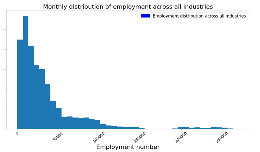
plt.figure(figsize=(16,8))
plt.hist(data_output['Employment'], bins =40)
#plt.plot(years[0], retail_series['Employment'], color = 'b',marker='o', linewidth=1)

plt.xlabel('Employment number', fontsize=22)
plt.xticks(rotation=40, fontsize = 14)
#plt.ylabel('Other manufacturing  VS  Other retail', fontsize=22)
plt.yticks(fontsize = 0.1)
plt.title('Monthly distribution of employment across all industries', fontsize=22)
#red = patches.Patch(color='blue', label='Other manufacturing')
blue = patches.Patch(color='blue', label='Employment distribution across all industries')
plt.legend(handles=[blue], prop = {'size':15})
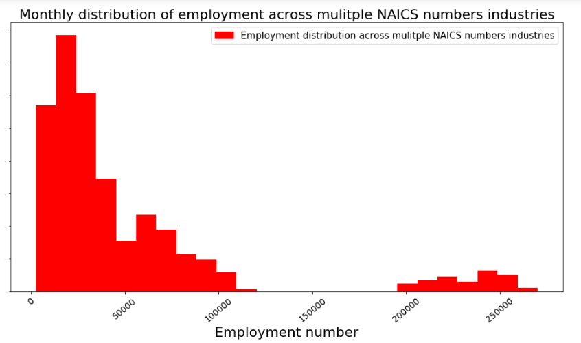
5. What is the monthly distribution of employment of mulitple NAICS numbers industries VS single NAICS number industries?
plt.figure(figsize=(16,8))
plt.hist(data_output_mixed['Employment'], bins = 25, color = 'r')
#plt.plot(years[0], retail_series['Employment'], color = 'b',marker='o', linewidth=1)

plt.xlabel('Employment number', fontsize=22)
plt.xticks(rotation=40, fontsize = 14)
#plt.ylabel('Other manufacturing  VS  Other retail', fontsize=22)
plt.yticks(fontsize = 0.1)
plt.title('Monthly distribution of employment across mulitple NAICS numbers industries', fontsize=22)
#red = patches.Patch(color='blue', label='Other manufacturing')
blue = patches.Patch(color='red', label='Employment distribution across mulitple NAICS numbers industries')
plt.legend(handles=[blue], prop = {'size':15})
Data Source : Labour Force Survey (LFS) by the Statistics of Canada.
This project is done as a part of Data Insight program assignment.

















תגובות